Recurrence Relation

Recurance Relation

A recurrence is an equation or inequality that describes a function in terms of its values on smaller inputs. To solve a Recurrence Relation means to obtain a function defined on the natural numbers that satisfy the recurrence.

For Example, the Worst Case Running Time T(n) of the MERGE SORT Procedures is described by the recurrence.

T (n) = θ (1) if n=1 2T + θ (n) if n>1

There are four methods for solving Recurrence:

1. Substitution Method
2. Iteration Method
3. Recursion Tree Method
4. Master Method

---

1. Substitution Method:

The Substitution Method Consists of two main steps:

1. Guess the Solution.
2. Use the mathematical induction to find the boundary condition and shows that the guess is correct.

For Example1 Solve the equation by Substitution Method.

T (n) = T![DAA Recurrence Relation](https://static.javatpoint.com/tutorial/daa/images/daa-recurrence-relation.png) + n

We have to show that it is asymptotically bound by O (log n).

Solution:

For T (n) = O (log n)

We have to show that for some constant c

1. T (n) ≤c logn.

Put this in given Recurrence Equation.

T (n) ≤c log![DAA Recurrence Relation](https://static.javatpoint.com/tutorial/daa/images/daa-recurrence-relation.png)+ 1
        ≤c log![DAA Recurrence Relation](https://static.javatpoint.com/tutorial/daa/images/daa-recurrence-relation.png)+ 1 = c logn-clog2 2+1
        ≤c logn for c≥1

Thus T (n) =O logn.

Example2 Consider the Recurrence

T (n) = 2T+ n n>1

Find an Asymptotic bound on T.

Solution:

We guess the solution is O (n (logn)).Thus for constant 'c'. T (n) ≤c n logn Put this in given Recurrence Equation. Now, T (n) ≤2clog +n ≤cnlogn-cnlog2+n =cn logn-n (clog2-1) ≤cn logn for (c≥1) Thus T (n) = O (n logn).

---

2. Iteration Methods

It means to expand the recurrence and express it as a summation of terms of n and initial condition.

Example1: Consider the Recurrence

1. T (n) = 1 if n=1
2. = 2T (n-1) if n>1

Solution:

T (n) = 2T (n-1) = 2[2T (n-2)] = 22T (n-2) = 4[2T (n-3)] = 23T (n-3) = 8[2T (n-4)] = 24T (n-4) (Eq.1)

Repeat the procedure for i times

T (n) = 2i T (n-i) Put n-i=1 or i= n-1 in (Eq.1) T (n) = 2n-1 T (1) = 2n-1 .1 {T (1) =1 .....given} = 2n-1

Example2: Consider the Recurrence

1. T (n) = T (n-1) +1 and T (1) = θ (1).

Solution:

T (n) = T (n-1) +1 = (T (n-2) +1) +1 = (T (n-3) +1) +1+1 = T (n-4) +4 = T (n-5) +1+4 = T (n-5) +5= T (n-k) + k Where k = n-1 T (n-k) = T (1) = θ (1) T (n) = θ (1) + (n-1) = 1+n-1=n= θ (n).

Solutions of recurrence relations by Master Methods

The Master Method is used for solving the following types of recurrence

T (n) = a T+ f (n) with a≥1 and b≥1 be constant & f(n) be a function and can be interpreted as

Let T (n) is defined on non-negative integers by the recurrence.

T (n) = a T+ f (n)

In the function to the analysis of a recursive algorithm, the constants and function take on the following significance:

• n is the size of the problem.
• a is the number of subproblems in the recursion.
• n/b is the size of each subproblem. (Here it is assumed that all subproblems are essentially the same size.)
• f (n) is the sum of the work done outside the recursive calls, which includes the sum of dividing the problem and the sum of combining the solutions to the subproblems.
• It is not possible always bound the function according to the requirement, so we make three cases which will tell us what kind of bound we can apply on the function.

Master Theorem:

It is possible to complete an asymptotic tight bound in these three cases:

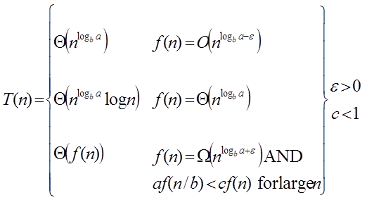
Case1: If f (n) = for some constant ε >0, then it follows that:

T (n) = Θ

Example:

T (n) = 8 T apply master theorem on it.

Solution:

Compare T (n) = 8 T with T (n) = a T a = 8, b=2, f (n) = 1000 n2, logba = log28 = 3 Put all the values in: f (n) = 1000 n2 = O (n3-ε ) If we choose ε=1, we get: 1000 n2 = O (n3-1) = O (n2)

Since this equation holds, the first case of the master theorem applies to the given recurrence relation, thus resulting in the conclusion:

T (n) = Θ Therefore: T (n) = Θ (n3)

Case 2: If it is true, for some constant k ≥ 0 that:

F (n) = Θ then it follows that: T (n) = Θ

Example:

T (n) = 2 , solve the recurrence by using the master method. As compare the given problem with T (n) = a T a = 2, b=2, k=0, f (n) = 10n, logba = log22 =1 Put all the values in f (n) =Θ , we will get 10n = Θ (n1) = Θ (n) which is true. Therefore: T (n) = Θ = Θ (n log n)

Case 3: If it is true f(n) = Ω for some constant ε >0 and it also true that: a f for some constant c<1 for large value of n ,then :

1. T (n) = Θ((f (n))

Example: Solve the recurrence relation:

T (n) = 2

Solution:

Compare the given problem with T (n) = a T a= 2, b =2, f (n) = n2, logba = log22 =1 Put all the values in f (n) = Ω ..... (Eq. 1) If we insert all the value in (Eq.1), we will get n2 = Ω(n1+ε) put ε =1, then the equality will hold. n2 = Ω(n1+1) = Ω(n2) Now we will also check the second condition: 2 If we will choose c =1/2, it is true: ∀ n ≥1 So it follows: T (n) = Θ ((f (n)) T (n) = Θ(n2)

Divide and Conquer

To understand the divide and conquer design strategy of algorithms, let us use a simple real world example. Consider an instance where we need to brush a type C curly hair and remove all the knots from it. To do that, the first step is to section the hair in smaller strands to make the combing easier than combing the hair altogether. The same technique is applied on algorithms.

Divide and conquer approach breaks down a problem into multiple sub-problems recursively until it cannot be divided further. These sub-problems are solved first and the solutions are merged together to form the final solution.

The common procedure for the divide and conquer design technique is as follows −

• Divide − We divide the original problem into multiple sub-problems until they cannot be divided further.

• Conquer − Then these subproblems are solved separately with the help of recursion

• Combine − Once solved, all the subproblems are merged/combined together to form the final solution of the original problem.

There are several ways to give input to the divide and conquer algorithm design pattern. Two major data structures used are − arrays and linked lists. Their usage is explained as

Arrays as Input

There are various ways in which various algorithms can take input such that they can be solved using the divide and conquer technique. Arrays are one of them. In algorithms that require input to be in the form of a list, like various sorting algorithms, array data structures are most commonly used.

In the input for a sorting algorithm below, the array input is divided into subproblems until they cannot be divided further.

Then, the subproblems are sorted (the conquer step) and are merged to form the solution of the original array back (the combine step).

Since arrays are indexed and linear data structures, sorting algorithms most popularly use array data structures to receive input.

Binary Search Algorithm

Binary search is a fast search algorithm with run-time complexity of Ο(log n). This search algorithm works on the principle of divide and conquer, since it divides the array into half before searching. For this algorithm to work properly, the data collection should be in the sorted form.

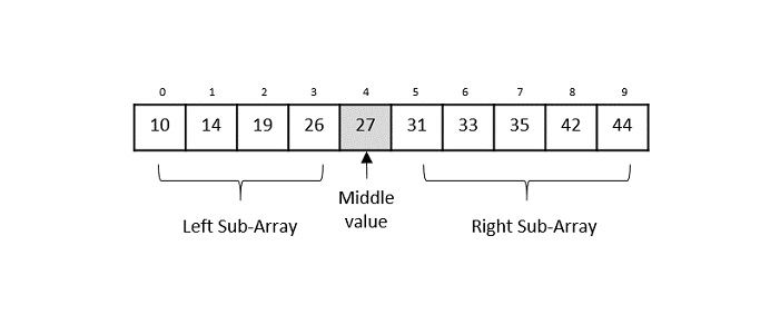
Binary search looks for a particular key value by comparing the middle most item of the collection. If a match occurs, then the index of item is returned. But if the middle item has a value greater than the key value, the right sub-array of the middle item is searched. Otherwise, the left sub-array is searched. This process continues recursively until the size of a subarray reduces to zero.

Binary Search Algorithm

Binary Search algorithm is an interval searching method that performs the searching in intervals only. The input taken by the binary search algorithm must always be in a sorted array since it divides the array into subarrays based on the greater or lower values. The algorithm follows the procedure below −

Step 1 − Select the middle item in the array and compare it with the key value to be searched. If it is matched, return the position of the median.

Step 2 − If it does not match the key value, check if the key value is either greater than or less than the median value.

Step 3 − If the key is greater, perform the search in the right sub-array; but if the key is lower than the median value, perform the search in the left sub-array.

Step 4 − Repeat Steps 1, 2 and 3 iteratively, until the size of sub-array becomes 1.

Step 5 − If the key value does not exist in the array, then the algorithm returns an unsuccessful search.

Pseudocode

The pseudocode of binary search algorithms should look like this −

Procedure binary_search A ← sorted array n ← size of array x ← value to be searched

Set lowerBound = 1 Set upperBound = n

while x not found if upperBound < lowerBound EXIT: x does not exists.

  set midPoint = lowerBound + ( upperBound - lowerBound ) / 2

  if A[midPoint] < x
     set lowerBound = midPoint + 1

  if A[midPoint] > x
     set upperBound = midPoint - 1

  if A[midPoint] = x
     EXIT: x found at location midPoint

end while end procedure

Analysis

Since the binary search algorithm performs searching iteratively, calculating the time complexity is not as easy as the linear search algorithm.

The input array is searched iteratively by dividing into multiple sub-arrays after every unsuccessful iteration. Therefore, the recurrence relation formed would be of a dividing function.

Quick sort

It is an algorithm of Divide & Conquer type.

Divide: Rearrange the elements and split arrays into two sub-arrays and an element in between search that each element in left sub array is less than or equal to the average element and each element in the right sub- array is larger than the middle element.

Conquer: Recursively, sort two sub arrays.

Combine: Combine the already sorted array.

Algorithm:

1. QUICKSORT (array A, int m, int n)
2. 1 if (n > m)
3. 2 then
4. 3 i ← a random index from [m,n]
5. 4 swap A [i] with A[m]
6. 5 o ← PARTITION (A, m, n)
7. 6 QUICKSORT (A, m, o - 1)
8. 7 QUICKSORT (A, o + 1, n)

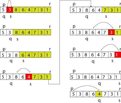
Partition Algorithm:

Partition algorithm rearranges the sub arrays in a place.

1. PARTITION (array A, int m, int n)
2. 1 x ← A[m]
3. 2 o ← m
4. 3 for p ← m + 1 to n
5. 4 do if (A[p] < x)
6. 5 then o ← o + 1
7. 6 swap A[o] with A[p]
8. 7 swap A[m] with A[o]
9. 8 return o

Figure: shows the execution trace partition algorithm

Merge Sort Algorithm

In this article, we will discuss the merge sort Algorithm. Merge sort is the sorting technique that follows the divide and conquer approach. This article will be very helpful and interesting to students as they might face merge sort as a question in their examinations. In coding or technical interviews for software engineers, sorting algorithms are widely asked. So, it is important to discuss the topic.

Merge sort is similar to the quick sort algorithm as it uses the divide and conquer approach to sort the elements. It is one of the most popular and efficient sorting algorithm. It divides the given list into two equal halves, calls itself for the two halves and then merges the two sorted halves. We have to define the merge() function to perform the merging.

The sub-lists are divided again and again into halves until the list cannot be divided further. Then we combine the pair of one element lists into two-element lists, sorting them in the process. The sorted two-element pairs is merged into the four-element lists, and so on until we get the sorted list.

Now, let's see the algorithm of merge sort.

Algorithm

In the following algorithm, arr is the given array, beg is the starting element, and end is the last element of the array.

1. MERGE_SORT(arr, beg, end)

2. if beg < end

3. set mid = (beg + end)/2
4. MERGE_SORT(arr, beg, mid)
5. MERGE_SORT(arr, mid + 1, end)
6. MERGE (arr, beg, mid, end)

7. end of if

8. END MERGE_SORT

The important part of the merge sort is the MERGE function. This function performs the merging of two sorted sub-arrays that are A[beg…mid] and A[mid+1…end], to build one sorted array A[beg…end]. So, the inputs of the MERGE function are A[], beg, mid, and end.

The implementation of the MERGE function is given as follows -

1. / Function to merge the subarrays of a[] /
2. void merge(int a[], int beg, int mid, int end)
3. {
4. int i, j, k;
5. int n1 = mid - beg + 1;

6. int n2 = end - mid;

7. int LeftArray[n1], RightArray[n2]; //temporary arrays

8. / copy data to temp arrays /

9. for (int i = 0; i < n1; i++)
10. LeftArray[i] = a[beg + i];
11. for (int j = 0; j < n2; j++)

12. RightArray[j] = a[mid + 1 + j];

13. i = 0, / initial index of first sub-array /

14. j = 0; / initial index of second sub-array /

15. k = beg; / initial index of merged sub-array /

16. while (i < n1 && j < n2)

17. {
18. if(LeftArray[i] <= RightArray[j])
19. {
20. a[k] = LeftArray[i];
21. i++;
22. }
23. else
24. {
25. a[k] = RightArray[j];
26. j++;
27. }
28. k++;
29. }
30. while (i<n1)
31. {
32. a[k] = LeftArray[i];
33. i++;
34. k++;

35. }

36. while (j<n2)

37. {
38. a[k] = RightArray[j];
39. j++;
40. k++;
41. }
42. }

Working of Merge sort Algorithm

Now, let's see the working of merge sort Algorithm.

To understand the working of the merge sort algorithm, let's take an unsorted array. It will be easier to understand the merge sort via an example.

Let the elements of array are -

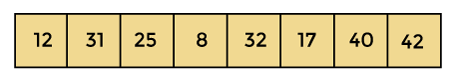
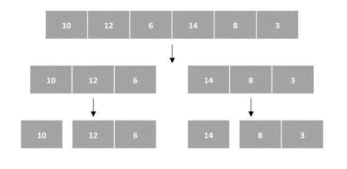
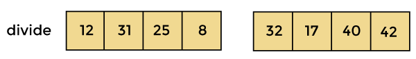
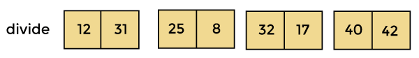
According to the merge sort, first divide the given array into two equal halves. Merge sort keeps dividing the list into equal parts until it cannot be further divided.

As there are eight elements in the given array, so it is divided into two arrays of size 4.

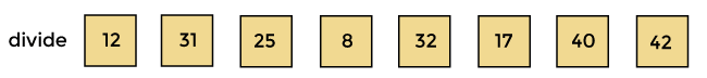
Now, again divide these two arrays into halves. As they are of size 4, so divide them into new arrays of size 2.

Now, again divide these arrays to get the atomic value that cannot be further divided.

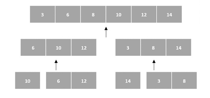
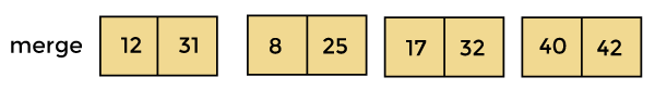
Now, combine them in the same manner they were broken.

In combining, first compare the element of each array and then combine them into another array in sorted order.

So, first compare 12 and 31, both are in sorted positions. Then compare 25 and 8, and in the list of two values, put 8 first followed by 25. Then compare 32 and 17, sort them and put 17 first followed by 32. After that, compare 40 and 42, and place them sequentially.

In the next iteration of combining, now compare the arrays with two data values and merge them into an array of found values in sorted order.

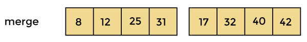
Now, there is a final merging of the arrays. After the final merging of above arrays, the array will look like -

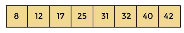
Now, the array is completely sorted.

Merge sort complexity

Now, let's see the time complexity of merge sort in best case, average case, and in worst case. We will also see the space complexity of the merge sort.

1. Time Complexity

Case	Time Complexity
Best Case	O(n * log n)
Average Case	O(n * log n)
Worst Case	O(n * log n)

• Best Case Complexity - It occurs when there is no sorting required, i.e. the array is already sorted. The best-case time complexity of merge sort is O(n*logn).
• Average Case Complexity - It occurs when the array elements are in jumbled order that is not properly ascending and not properly descending. The average case time complexity of merge sort is O(n*logn).
• Worst Case Complexity - It occurs when the array elements are required to be sorted in reverse order. That means suppose you have to sort the array elements in ascending order, but its elements are in descending order. The worst-case time complexity of merge sort is O(n*logn).

2. Space Complexity

Property	Value
Space Complexity	O(n)
Stable	YES

• The space complexity of merge sort is O(n). It is because, in merge sort, an extra variable is required for swapping.

Maximum and Minimum finding

Let us consider a simple problem that can be solved by divide and conquer technique.

Maximum and Minimum finding

The Max-Min Problem in algorithm analysis is finding the maximum and minimum value in an array.

Solution

To find the maximum and minimum numbers in a given array numbers[] of size n, the following algorithm can be used. First we are representing the naive method and then we will present divide and conquer approach.

Naive Method

Naive method is a basic method to solve any problem. In this method, the maximum and minimum number can be found separately. To find the maximum and minimum numbers, the following straightforward algorithm can be used.

Algorithm: Max-Min-Element (numbers[]) max := numbers[1] min := numbers[1]

for i = 2 to n do if numbers[i] > max then
max := numbers[i] if numbers[i] < min then
min := numbers[i] return (max, min)

Example

Following are the implementations of the above approach in various programming languages −

C

include

struct Pair { int max; int min; }; // Function to find maximum and minimum using the naive algorithm struct Pair maxMinNaive(int arr[], int n) { struct Pair result; result.max = arr[0]; result.min = arr[0]; // Loop through the array to find the maximum and minimum values for (int i = 1; i < n; i++) { if (arr[i] > result.max) { result.max = arr[i]; // Update the maximum value if a larger element is found } if (arr[i] < result.min) { result.min = arr[i]; // Update the minimum value if a smaller element is found } } return result; // Return the pair of maximum and minimum values } int main() { int arr[] = {6, 4, 26, 14, 33, 64, 46}; int n = sizeof(arr) / sizeof(arr[0]); struct Pair result = maxMinNaive(arr, n); printf("Maximum element is: %d\n", result.max); printf("Minimum element is: %d\n", result.min); return 0; }

Output

Maximum element is: 64 Minimum element is: 4

Reference

https://www.javatpoint.com/daa-recurrence-relation https://www.javatpoint.com/daa-master-method https://www.tutorialspoint.com/data_structures_algorithms/divide_and_conquer.htm https://www.tutorialspoint.com/design_and_analysis_of_algorithms/design_and_analysis_of_algorithms_binary_search_method.htm https://www.javatpoint.com/daa-quick-sort https://www.javatpoint.com/merge-sort https://www.tutorialspoint.com/design_and_analysis_of_algorithms/design_and_analysis_of_algorithms_max_min_problem.htm